Sentiment Symposium Tutorial: Lexicons

1. Overview
2. Resources
   1. Bing Liu's Opinion Lexicon
   2. MPQA Subjectivity Lexicon
   3. SentiWordNet
   4. Harvard General Inquirer
   5. LIWC
   6. Relationships
3. Building your own lexicons
   1. Simple WordNet propagation
   2. Weighted WordNet propagation
   3. Review word scores
      1. Data
      2. Category sizes
      3. Word distributions: Raw counts are misleading
      4. Word distributions: Relative frequencies
      5. Word distributions: Probabilities
      6. Scoring with expected ratings
      7. Scoring with logistic regression
   4. Experience Project reaction distributions
      1. Data
      2. Word distributions: Observed and expected counts
4. Summary of conclusions

Overview

Many sentiment applications rely on lexicons to supply features to a model. This section reviews some publicly available resources and their relationships, and it seeks to identify some best practices for using sentiment lexicons effectively.

Resources

Bing Liu's Opinion Lexicon

Bing Liu maintains and freely distributes a sentiment lexicon consisting of lists of strings.

• Distribution page (direct link to rar archive)
• Positive words: 2006
• Negative words: 4783
• Useful properties: includes mis-spellings, morphological variants, slang, and social-media mark-up

MPQA Subjectivity Lexicon

The MPQA (Multi-Perspective Question Answering) Subjectivity Lexicon is maintained by Theresa Wilson, Janyce Wiebe, and Paul Hoffmann (Wiebe, Wilson, and Cardie 2005). It is distributed under a GNU Public License. Table tab:mpqa shows what its structure is like.

SentiWordNet

SentiWordNet (note: this site was hacked recently; take care when visiting it) (Baccianella, Esuli, and Sebastiani 2010) attaches positive and negative real-valued sentiment scores to WordNet synsets (Fellbaum1998). It is freely distributed for noncommercial use, and licensed are available for commercial applications. (See the website for details.) Table tab:sentiwordnet summarizes its structure. (For extensive discussion of WordNet synsets and related objects, see this introduction).

Harvard General Inquirer

The Harvard General Inquirer is a lexicon attaching syntactic, semantic, and pragmatic information to part-of-speech tagged words (Stone, Dunphry, Smith, and Ogilvie 1966). The spreadsheet format is the easiest one to work with for most computational applications. Table tab:inquirer provides a glimpse of the richness and complexity of this resource.

LIWC

Linguistic Inquiry and Word Counts (LIWC) is a propriety database consisting of a lot of categorized regular expressions. It costs about $90. Its classifications are highly correlated with those of the Harvard General Inquirer. Table tab:liwc gives some of its sentiment-relevant categories with example regular expressions.

Relationships

All of the above lexicons provide basic polarity classifications. Their underlying vocabularies are different, so it is difficult to compare them comprehensively, but we can see how often they explicitly disagree with each other in that they supply opposite polarity values for a given word. Table tab:lexicon_disagreement reports on the results of such comparisons.

(Where a lexicon had part-of-speech tags, I removed them and selected the most sentiment-rich sense available for the resulting string. For SentiWordNet, I counted a word as positive if its positive score was larger than its negative score; negative if its negative score was larger than its positive score; else neutral, which means that words with equal non-0 positive and negative scores are neutral.)

I can imagine two equally reasonable reaction to the disagreements. The first would be to resolve them in favor of some particular sense. The second would be to combine the values derived from theses resources, thereby allowing the conflicts to persist, as a way of capturing the fact that the disagreements arise from genuine sense ambiguities.

Building your own lexicons

The above lexicons are useful for a wide range of tasks, but they are fixed resources. This section is devoted to developing new resources. This can have three benefits, which we will see in various combinations:

1. Much larger lexicons can be developed inferentially.
2. We can capture different dimensions of sentiment that might be pressing for specific tasks.
3. We can develop lexicons that are sensitive to the norms of specific domains.

Simple WordNet propagation

The guiding idea behind simple WordNet propagation is the properties of some hand-selected seed-sets will be preserved as we travel strategically through WordNet (Hu and Liu 2004 Andreevskaia and Bergler 2006 Esuli and Sebastiani 2006 Kim and Hovy 2006 Godbole, Srinivasaiah, and Skiena 2007 Rao and Ravichandran 2009).

The algorithm begins with n small, hand-crafted seed-sets and then follows WordNet relations from them, thereby expanding their size. The expanded sets of iteration i are used as seed-sets for iteration i+1, generally after pruning any pairwise overlap between them.

The algorithm is spelled out in full in figure fig:wnpropagate.

Figure fig:wnpropagate

Free hyper parameters: the seed-sets, the WordNet relations called in SamePolarity and OtherPolarity, the number of iterations, the decision to remove overlap.

The algorithm has a number of free parameters: the seed-sets, the WordNet relations called in SamePolarity and OtherPolarity, the number of iterations, the decision to remove overlap. The demo allows you to try out different combinations of values:

Table tab:wnpropagate_exs provides some additional seed-sets, drawing from other distinctions found in the Harvard Inquirer. These can be pasted into the demo if one wants a sense for how well new lexical classes propagate.

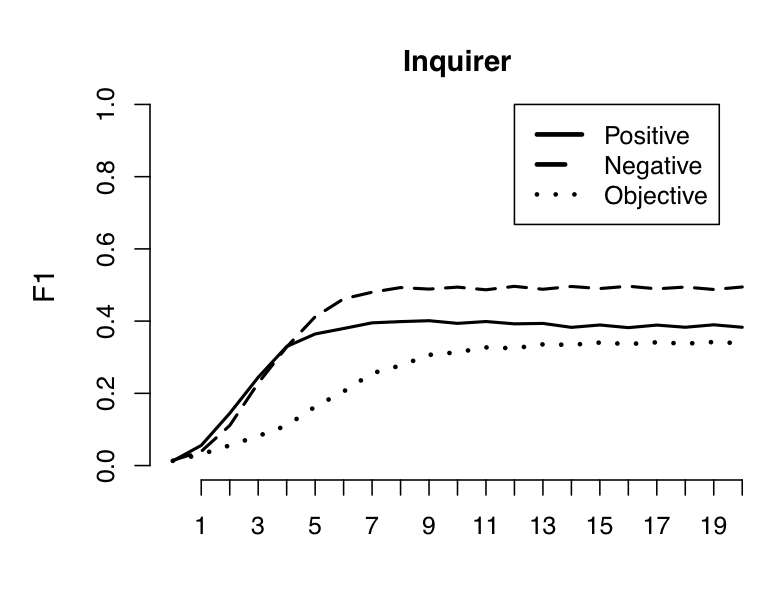
To assess the algorithm for polarity sense-preservation, I began with the seed-sets in table tab:seeds and then allowed the propagation algorithm to run for 20 iterations, checking each for its effectiveness at reproducing the Positiv/Negativ/Neither distinctions in the subset of Harvard General Inquirer that is also in WordNet.

Figure fig:wnpropagate-assess summarizes the results of this experiment, which are decidedly mixed.

Figure fig:wnpropagate-assess

Assessing how well simple Wordnet propagation is able to recover the Harvard Inquirer Positiv/Negativ/Neither classes using the seed sets of table tab:seeds.

Weighted WordNet propagation

Blair-Goldensohn, Hannan, McDonald, Ryan, Reis, and Reynar (2008) developed an algorithm that propagates not only the senses of the original seed set but also attaches scores to words, reflecting their intensity, which here is given by the strength of their graphical connections to the seed words. The algorithm is stated in figure fig:wnscores_algorithm.

Figure fig:wnscores_algorithm

The WordNet score propagation algorithm.

Figure fig:wnscores_example works through an example.

Figure fig:wnscores_example

WordNet score propagation example. The authors propose a further rescaling of the scores: log(abs(s)) * sign(s) if abs(s) > 1, else 0. However, in the example, we would lose the sentiment score for good if we stopped before iteration 6. In my experiments, rescaling resulted in dramatically fewer non-0 values.

I ran the algorithm using the full Harvard General Inquirer Positiv/Negative/Neither classes as seeds-sets. The output in archived CSV format:

• WordNet scores lexicon (zip file)
• Associated readme file (txt file)

You can view the results at the lexicon demo.

In my informal assessment, the positive and negative scores it assigns tend to be accurate. The disappointment is that so many of the scores are 0, as see in figure fig:wnscores_scoredist. I think this could be addressed by following more relations that just the basic synset one, as we do for the simple WordNet propagation algorithm, but I've not tried it yet.

Figure fig:wnscores_scoredist

WordNet score propagation score distribution.

Review word scores

In this section, I make use of the CSV-formatted data here:

• http://compprag.christopherpotts.net/code-data/imdb-words.csv.zip

This is a tightly controlled, POS-tagged dataset. Even more carefully curated ones are here, drawing from a wider range of corpora:

• http://www.stanford.edu/~cgpotts/data/wordnetscales/

And for more naturalistic, non-POS-tagged data in this format from a variety of sources:

• http://www.stanford.edu/~cgpotts/data/salt20/potts-salt20-data-and-code.zip

The methods are discussed and motivated in Constant, Davis, Potts, and Schwarz 2008 and Potts and Schwarz 2010, and this page provides a more extended discussion with associated R code.

Data

The file http://compprag.christopherpotts.net/code-data/imdb-words.csv.zip consists of data gathered from the user-supplied reviews at the IMDB. I suggest that you take a moment right now to browse around the site a bit to get a feel for the nature of the reviews — their style, tone, and so forth.

The focus of this section is the relationship between the review authors' language and the star ratings they choose to assign, from the range 1-10 stars (with the exception of This is Spinal Tap, which goes to 11). Intuitively, the idea is that the author's chosen star rating affects, and is affected by, the text she produces. The star rating is a particular kind of high-level summary of the evaluative aspects of the review text, and thus we can use that high-level summary to get a grip on what's happening linguistically.

The data I'll be working with are all in the format described in table tab:data. Each row represents a star-rating category. Thus, for example, in these data, (bad, a) is used 122,232 in 1-star reviews, and the total token count for 1-star reviews is 25,395,214.

The next few sections describe methods for deriving sentiment lexicons from such data. The methods should generalize to other kinds of ordered sentiment metadata (e.g., helpfulness ratings, confidence ratings).

Category sizes

A common feature of online user-supplied reviews is that the positive reviews vastly out-number the negative ones; see figure fig:totals.

Figure fig:totals

The highly imbalanced category sizes.

Word distributions: Raw counts are misleading

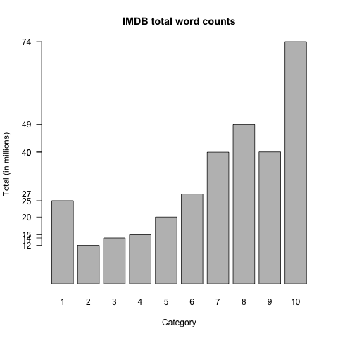
As we saw above, the raw Count values are likely to be misleading due to the very large size imbalances among the categories. For example, there are more tokens of (bad, a) in 10-star reviews than in 2-star ones, which seems highly counter-intuitive. Plotting the values reveals that the Count distribution is very heavily influenced by the overall distribution of words (figure fig:counts).

Figure fig:counts

Count distribution for (bad, a) (left) and the overall category size (right; repeated from figure fig:totals). The distribution is heavily influenced by the category sizes.

The source of this odd picture is clear: the 10-star category is 7 times bigger than the 1-star category, so the absolute counts do not necessarily reflect the rate of usage.

Word distributions: Relative frequencies

To get a better read on the usage patterns, we use relative frequencies:

Definition: Relative Frequencies (RelFreq)

Count/Total

Table tab:relfreq extends table tab:data with these RelFreq values.

Relative frequency values are hard to get a grip on intuitively because they are so small. Plotting helps bring out the relationships between the values, as in figure fig:relfreq.

Figure fig:relfreq

RelFreq distribution for (bad, a) (left), alongside the Count distribution (right; repeated from figure fig:counts). RelFreq values show little or no influence from the underlying category sizes.

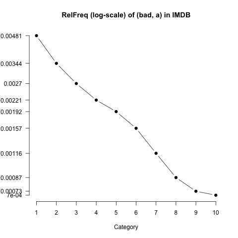
One drawback to RelFreq values is that they are highly sensitive to overall frequency. For example, (bad, a) is significantly more frequent than (horrible, a), which means that the RelFreq values for the two words are hard to directly compare. Figure fig:relfreq_cmp nonetheless attempts a comparison.

Figure fig:relfreq_cmp

Comparing words via their RelFreq distributions.

It is possible to discern that (bad, a) is less extreme in its negativity than (horrible, a). However, the effect looks subtle. The next measure we look at abstracts away from overall frequency, which facilitates this kind of direct comparison.

Word distributions: Probabilities

A drawback to RelFreq values, at least for present purposes, is that they are extremely sensitive to the overall frequency of the word in question. There is a comparable value that is insensitive to this quantity:

Definition: Pr values

RelFreq / sum(RelFreq)

Pr values are just rescaled RelFreq values: we divide by a constant to get from RelFreq to Pr. As a result, the distributions have exactly the same shape, as we see in figure fig:pr.

Figure fig:pr

Comparing Pr values (left) with RelFreq values (right; repeated from figure fig:relfreq). The shapes are exactly the same (Pr is a rescaling of RelFreq).

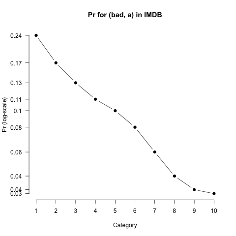
A technical note: The move from RelFreq to Pr involves an application of Bayes Rule.

1. RelFreq Values can be thought of as estimates of the conditional distribution P(word|rating): given that I am in rating category rating, how likely am I to produce word?
2. Bayes Rule allows us to obtain the inverse distribution P(rating|word):
   P(rating|word) = P(word|rating)P(rating) / P(word)
3. However, we would not want to directly apply this rule, because of the term P(rating) in the numerator. That would naturally be approximated by the distribution given by Total, as in figure fig:totals, which would simply re-introduce all of those unwanted biases.
4. Thus, we keep P(rating) constant, which is just to say that we leave it out:
   P(word|rating) / P(word)
   where P(word) = sum(RelFreq).

Pr values greatly facilitate comparisons between words (figure fig:pr_cmp).

Figure fig:pr_cmp

Comparing the Pr distributions of (bad, a) and (horrible, a). The comparison is easier than it was with RelFreq values (figure fig:relfreq).

I think these plots clearly convey that (bad, a) is less intensely negative than (horrible, a). For example, whereas (bad, a) is at least used throughout the scale, even at the top, (horrible, a) is effectively never used at the top of the scale.

(For methods that rigorously compare word distributions of this sort, see this write-up, this talk, and Davis 2011.)

Scoring with expected ratings

We are now in a position to assign polarity scores to words. A first method for doing this uses expected ratings:

Definition: Expected ratings

sum((Category-5.5) * Pr)

Subtracting 5.5 from the Category values centers them at 0, so that we can treat scores below 0 as negative and scores above 0 as positive.

Expected ratings calculations are used by de Marneffe et al. 2010 to summarize Pr-based distributions. The expected rating calculation is just a weighted average of Pr values.

To get a feel for these values, it helps to work through some examples:

1. The rating vector is R = [-4.5 .. 4.5]
2. If the Pr is P = [0, 0, 0, 0, 0, 0, 0, 0, 0, 1] (all 10-star), then sum(R * P) = 4.5
3. If the rating vector is R = [0, 0, 0.2, 0, 0, 0, 0, 0, 0, 0.8] (all 10-star), then we do sum(R * P) = 3.1
4. If the rating vector is R = [1, 0, 0, 0, 0, 0, 0, 0, 0, 0] (all 10-star), then we do sum(R * P) = -4.5
5. If the rating vector is R = [0.35, 0.26, 0.1, 0.05, 0.05, 0.05, 0.02, 0.02, 0.05, 0.05] (all 10-star), then we do sum(R * P) = -2.33

Figure fig:er

Pr plots with added expected rating.

To get sentiment classification and intensity, we treat words with ER values below 0 as negative, those with ER valus above 0 as positive, and then use the absolute values as measures of intensity:

Definition: Sentiment lexicon via ER values.

A word w is positive if ER(w) ≥ 0, else negative.

A word w's intensity is abs(ER(w)).

Scoring with logistic regression

Expected ratings are easy to calculate and quite intuitive, but it is hard to know how confident we can be in them, because they are insensitive to the amount and kind of data that went into them. Suppose the ER for words v and w are both 10, but we have 500 tokens of v and just 10 tokens of w. This suggests that we can have a high degree of confidence in our ER for v, but not for w. However, ER values don't encode this uncertainty, nor is there an obvious way to capture it.

Logistic regression provides a useful way to do the work of ERs but with the added benefits of having a model and associated test statistics and measures of confidence. For our purposes, we can stick to a simple model that uses Category values to predict word usage. The intuition here is just the one that we have been working with so far: the star-ratings are correlated with the usage of some words. For a word like (bad, a), the correlation is negative: usage drops as the ratings get higher. For a word like (amazing, a), the correlation is positive.

With our logistic regression models, we will essentially fit lines through our RelFreq data points, just as one would with a linear regression involving one predictor. However, the logistic regression model fits these values in log-odds space and uses the inverse logit function (plogis in R) to ensure that all the predicted values lie in [0,1], i.e., that they are all true probability values. Unfortunately, there is not enough time to go into much more detail about the nature of this kind of modeling. I refer to Gelman and Hill  2008, §5-6 for an accessible, empirically-driven overview. Instead, let's simply fit a model and try to build up intuitions about what it does and says.

The simple linear regression model for bad is given in table tab:bad_fit. The model simply uses the rating values to predict the usage (log-odds) of the word in each category.

This model is plotted on figure fig:bad_fit.

Figure fig:bad_fit

RelFreq view of (bad, a) with logistic regression.

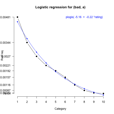
Here, we can use the coefficient for Category as our sentiment score. Where the value is negative (negative slope), the word is negative. Where it is positive, the word is positive. Informally, we can also use the size of the coefficient as a measure of its intensity.

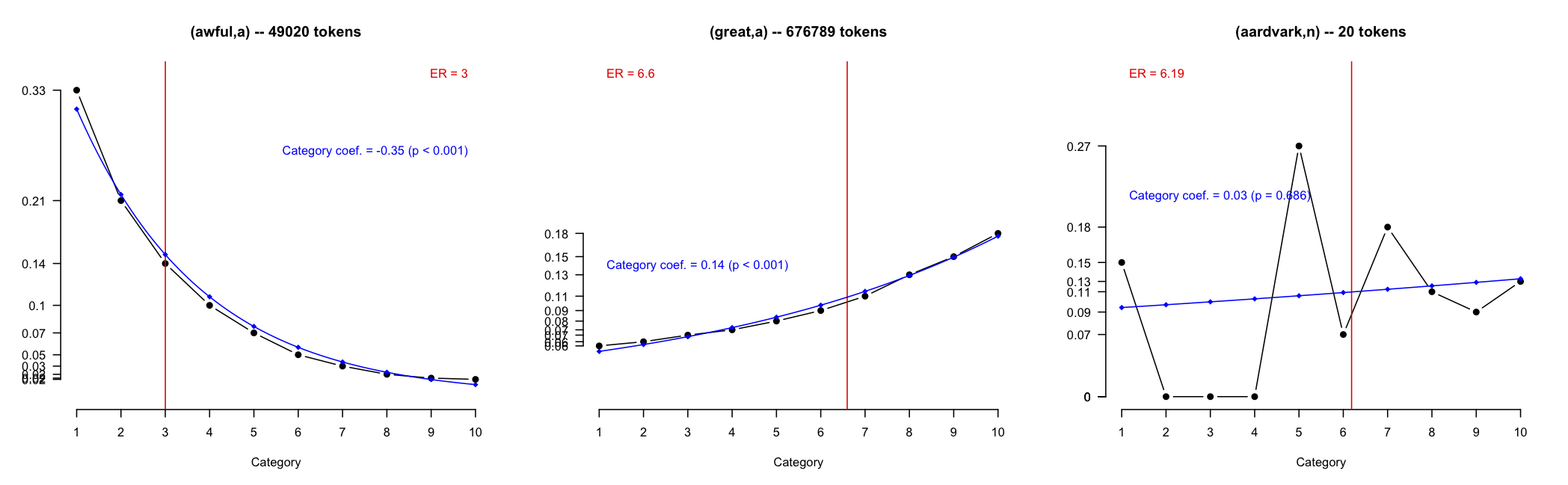
The great strength of this approach is that we can use the p-values to determine whether a score is trustworthy. Figure fig:cmp helps to convey why this is an important new power. (Here and in later plots, I've rescaled the values into Pr space to facilitate comparisons.)

Figure fig:cmp

Comparing words using our assessment values.

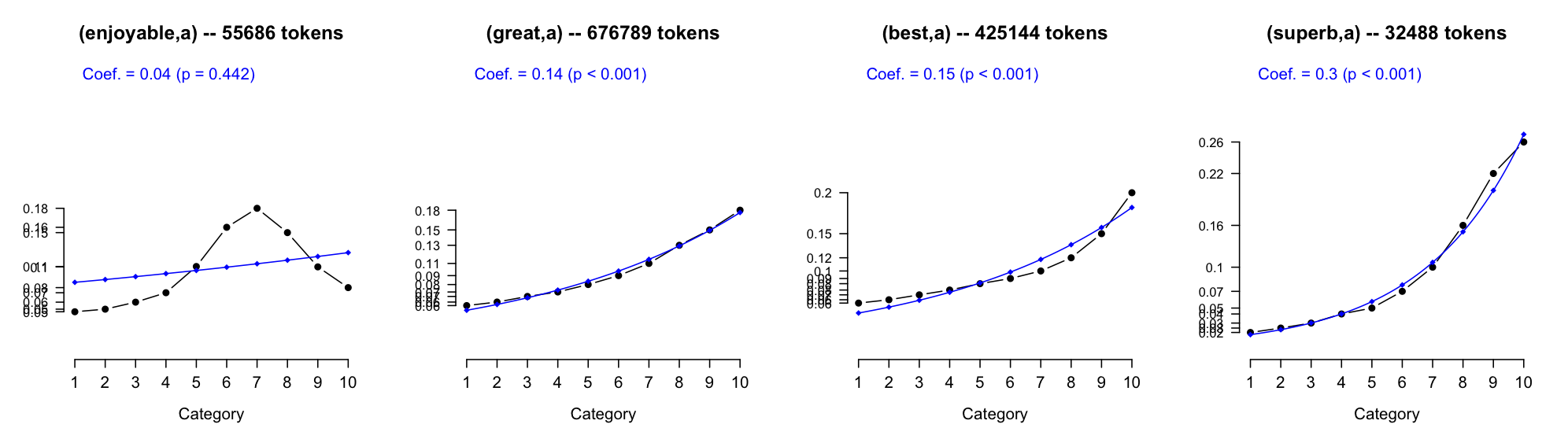
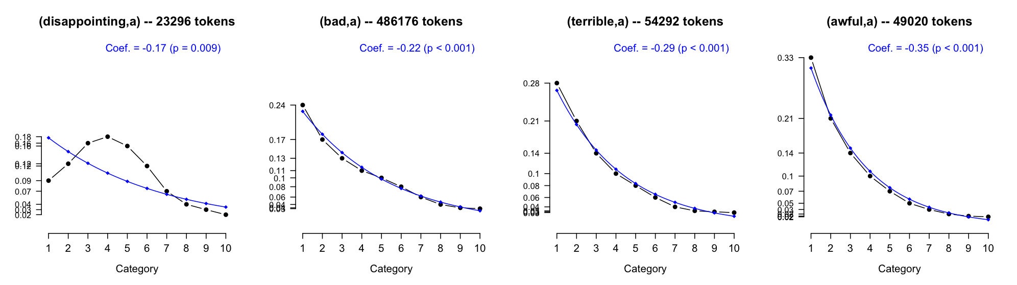
This leads to the following method for inducing a sentiment lexicon from these data:

Definition: Sentiment lexicon via logistic regression

Let Coef(w) be the Category coefficient for if that coefficient is significant at the chosen level, else 0

If Coef(w) = 0, then w is objective/neutral

If Coef(w) > 0, then w is positive

If Coef(w) < 0, then w is negative

A word's intensity is abs(Coef(w))

Depending on where the significance value is set, this can learn conservative lexicons of a few thousand words or very liberal lexicons of tens of thousands.

This method of comparing coefficient values is likely to irk statisticians, but it works well in practice. For a more exact and careful method, as well as a proposal for how to compare words with non-linear relationships to the ratings, see this talk I gave recently on creating lexical scales.

Figure fig:scalars shows off this new method of lexicon induction.

Figure fig:scalars

Some scalars in the IMDB.

Experience Project reaction distributions

The Experience Project is a social networking website that allows users to share stories about their own personal experiences. At the confessions portion of the site, users write typically very emotional stories about themselves, and readers can then chose from among five reaction categories to the story, but clicking on one of the five icons in figure fig:ep_cats. The categories provide rich new dimensions of sentiment, ones that are generally orthogonal to the positive/negative one that most people study but that nonetheless models important aspects of sentiment expression and social interaction (Potts 2010b, Socher, Pennington, Huang, Ng and Manning 2011).

Figure fig:ep_cats

Experience Project categories. "You rock" is a positive exclamative category. "Teehee" is a playful, lighthearted category. "I understand" is an expression of solidarity. "Sorry, hugs" is a sympathetic category. And "Wow, just wow" is negative exclamative, the least used category on the site.

This section presents a simple method for using these data to develop sentiment lexicons.

Data

As with the IMDB data above, I've put the word-level information into an easy-to-use CSV format, as in table tab:ep_data. Thus, as long as you require only word-level statistics, you needn't scrape the site again.

• Use the file epconfessions-unigrams.csv in http://www.stanford.edu/~cgpotts/data/salt20/potts-salt20-data-and-code.zip

Word distributions: Observed and expected counts

The basic scoring method contrasts observed click rates with expected click rates on the assumption that all word–click combinations are equally likely:

Definition: Observed/Expected values

Expected: sum(Count) / (Total/sum(Total))

The O/E values for w are Count/Expected

Table tab:oe extends table tab:ep_data with Expected and O/E values.

Some representative cases:

Figure fig:oe

O/E values for representative words.

These scores give rise to a multidimensional lexical entry via the following definition:

Definition: Multidimensional lexicon

EP(w) is a five dimensional vector of O/E values.

The Chi-squared test or the G-test (log-likelihood test) can be used to reduce these vectors to all-0 based on significance testing.

The lexicon demos include both IMDB and EP scores as well:

Summary of conclusions

1. There are a number of good fixed lexicons for sentiment. They are negligible to high levels of disagreement with each other. These can be exploited strategically — resolve the conflicts somehow or allow them to persist as genuine points of uncertainty.
2. WordNet can be used to derive interesting lexicons from small seeds sets, even for distinctions that are not directly encoded in WordNet's structure.
3. Naturally occurring metadata are a rich source of lexical entries. Statistical models are valuable for such lexicon induction.
4. A major advantage of inducing a lexicon directly from data is that one can then capture domain specific effects, which are very common in sentiment. (See also the discussion of vector-space models for lexicon induction methods that don't any metadata.)