Sentiment Symposium Tutorial: Vector-space models

1. Overview
2. Word–word matrices
3. Other matrix designs
4. Sentiment associates
5. Vector-based sentiment propagation
6. Related approaches
7. Summary of conclusions

Overview

This section introduces some basic techniques from the study of vector-space models. In the present setting, the guiding idea behind such models is that important aspects of a word's meanings are latent in its distribution, that is, in its patterns of co-occurrence with other words.

I focus on word–word matrices, rather than the more familiar and widely used word–document matrices of information retrieval and much of computational semantics. The reason for this is simply that, on the data I was experimenting with, this design seemed to be delivering better results with fewer resources.

Turney and Pantel 2010 is a highly readable introduction to vector-space models, covering a wide variety of different design choices and applications. I highly recommend it for anyone aiming to implement and deploy models like this.

Word–word matrices

A word–word for a vocabulary V of size n is an n × n matrix in which both the rows and columns represent words in V. The value in cell (i, j) is the number of times that word i and word j appear together in the same context.

Table tab:wordword depicts a fragment of a word–word matrix derived from 12,000 OpenTable reviews, using the sentiment + negation tokenization scheme motivated earlier. Here, the counts for (i, j) are the number of times that word i and word j appear together in the same review. With this matrix design, the rows and columns are the same, though they might be very different with other matrix designs.

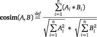
We now want to measure how similar the row vectors are to one another. If we compare the raw count vectors (say, by using Euclidean distance), then the dominating factor will be overall corpus frequency, which is unlikely to be sentiment relevant. Cosine similarity addresses this by comparing length normalized vectors:

Definition: Cosine similarity

The cosine similarity between vectors A and B of length n is

In table tab:cosine, I picked two sentiment rich target words, excellent and terrible, and compared them for cosine similarity against the whole vocabulary. The figure provides the 20 closest words by this similarity measure. Though the lists contain more function words than we might like, there are also rich sentiment words, some of them specific to the domain of restaurants, which suggest that we might use this method to increase our lexicon size in a context-dependent manner.

Singular value decomposition (SVD; see also the Latent Semantic Analysis of Deerwester, Dumais, Furnas, Landauer, and Harshman 1990) is a dimensionality reduction technique that has been shown to uncover a lot of underlying semantic structure. Table tab:svd shows the result of length normalizing the word–word matrix and then applying SVD to the result.

If we compare the new vectors, the results are somewhat different. To my eye, they look messier from a sentiment perspective. Going forward, I'll stick with the simpler method of just using cosine similarity on the raw count vectors.

Other matrix designs

There are many, many design choices available for vector-space models. We can vary not only the matrix itself but also the kinds of dimensionality reduction we perform (if any) and the similarity measures we employ. I refer to Turney and Pantel 2010 for a thorough overview. Here, I confine myself to mentioning a few other matrix designs that might be valuable for sentiment analysis:

• Word × document (very common)
• Word × word based on proximity in search engine results
• Word × word based on dependency edges
• Word × dependecy-edge
• Modifier × modified
• Twitter-based word × hashtag

Sentiment associates

Turney and Littman (2003) generalize the informal procedure used above, to achieve a general lexicon learning method. Their approach:

1. Given a word × context matrix, apply tf-idf weighting and then SVD.
2. Definite two seeds sets (positive vs. negative, or whatever contrast is of interest).
3. Rank words by their closeness to the seed sets, using the Semantic Orientation (SO) function defined just below.

Definition: Semantic orientation

Given opposing seeds sets S₁ and S₂, a matrix M, and a vector similarity measure vecSim defined for M, the semantic orientation of a word w is

Turney and Littman explore a number of different weighting schemes and similarity measures, paying special attention to how well they do on various corpus sizes. They conjecture that their approach can be generalized to a wide variety of sentiment contrasts.

I tried out a simple version of their approach on the OpenTable subset used above. The matrix was an unweighted word–word matrix, and the vector similarity measure was cosine similarity. The seed sets I used (table tab:so_seeds) are designed to aim for positive and negative words used to describe eating and good restaurant experiences. The top 20 positive and negative words are given in table tab:so. The results look extremely promising to me.

Vector-based sentiment propagation

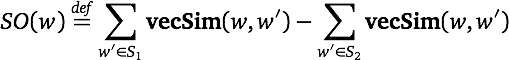
The method of Velikovich, Blair-Goldensohn, Hannan, and McDonald (2010) is closely related to that of Turney and Littman 2003, except that it extends the idea with a sophisticated and somewhat mind-bending propagation component aimed at learning truly massive sentiment lexicons.

The algorithm is defined in figure fig:webprop_algorithm.

Figure fig:webprop_algorithm

Web propagation algorithm. G is a cosine similarity graph. P and N are seed sets. γ is a threshold; sentiment scores below it are rounded to 0. T is the number of iterations.

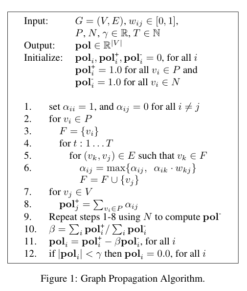
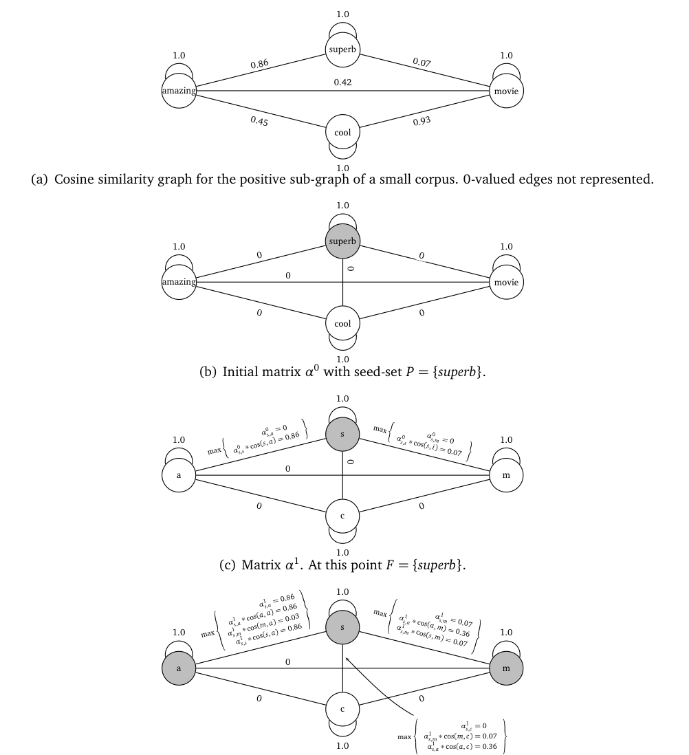
I use the simple example in table tab:webprop_ex illustrate how the algorithm works.

Figure fig:webprop_example continues the above example by showing how propagation works.

Figure fig:webprop_example

The iterative propagation method.

Velikovich et al. build a truly massive graph:

For this study, we used an English graph where the node set V was based on all n-grams up to length 10 extracted from 4 billion web pages. This list was filtered to 20 million candidate phrases using a number of heuristics including frequency and mutual information of word boundaries. A context vector for each candidate phrase was then constructed based on a window of size six aggregated over all mentions of the phrase in the 4 billion documents. The edge set $E$ was constructed by first, for each potential edge (v_i,v_j), computing the cosine similarity value between context vectors. All edges (v_i,v_j) were then discarded if they were not one of the 25 highest weighted edges adjacent to either node v_i or v_j.

Some highlights of their lexicon are given in figure fig:webprop_lexicon.

Figure fig:webprop_lexicon

Web prop lexicon

I think this approach is extremely promising, but I have not yet had the chance to try it out on sub-Google-sized corpora. However, I do have a small Python implementation for reference:

Related approaches

Once you have a distributional matrix, there are lots of things you can do with it:

1. Clustering
2. Topic modeling
3. Visualizations via 2d embedding

The central challenge for using these approaches in sentiment analysis is that they all tend to favor content-level associations over sentiment associations. That is, if you feed them the full vocabulary of your corpus, or the top n words from it, then you are unlikely to get sentiment-like groupings back. Some methods for addressing this challenge:

1. Filter the vocabulary to known sentiment words. (The drawback is that you won't learn any new ones.)
2. Filter the vocabulary to adjectives and adverbs. (The drawback is that you'll miss sentiment elsewhere.)
3. Bring in sentiment metadata to guide the unsupervised clustering model. This could be done with Labeled LDA (Ramage, Hall, Nallapati, and Manning 2009) or the related approach of Maas, Daly, Pham, Huang, Ng and Potts (2010), which is focused explicitly on learning sentiment-rich word vectors.

Summary of conclusions

1. Vector-space models seem to be capable of learning large and powerful feature sets capturing a variety of sentiment contrasts.
2. The number of design choices is dizzying, and there are relatively few proven guidelines, but this could be freeing, right?