Sentiment Symposium Tutorial: Classifiers

1. Overview
2. Models
   1. Naive Bayes
   2. Maximum Entropy
   3. Others
3. Assessing classifier models
   1. Accuracy and its limitations
   2. Precision
   3. Recall
   4. Derived effectiveness measures
   5. Training data assessment
   6. The importance of out-of-domain testing
4. Comparisons: Naive Bayes vs. MaxEnt
5. Feature selection
   1. A priori method cut-offs
   2. Lexicon induction as feature set induction
   3. Mutual information
   4. A cautionary note
6. Back the model competition
7. Tools
   1. The Stanford Classifier
   2. Others
8. A lightweight, accurate classifier
9. Summary of conclusions

Overview

This section introduces two classifier models, Naive Bayes and Maximum Entropy, and evaluates them in the context of a variety of sentiment analysis problems. Throughout, I emphasize methods for evaluating classifier models fairly and meaningfully, so that you can get an accurate read on what your systems and others' systems are really capturing.

Models

I concentrate on two closely related probabilistic models: Naive Bayes and MaxEnt. Some other classifier models are reviewed briefly below as well.

Naive Bayes

The Naive Bayes classifier is perhaps the simplest trained, probabilistic classifier model. It is remarkably effective in many situations.

I start by giving a recipe for training a Naive Bayes classifier using just the words as features:

1. Estimate the probability P(c) of each class c ∈ C by dividing the number of words in documents in c by the total number of words in the corpus.
2. Estimate the probability distribution P(w | c) for all words w and classes c. This can be done by dividing the number of tokens of w in documents in c by the total number of words in c.
3. To score a document d for class c, calculate
   
4. If you simply want to predict the most likely class label, then you can just pick the c with the highest score value. To get a probability distribution, calculate
   

The last step is important but often overlooked. The model predicts a full distribution over classes. Where the task is to predict a single label, one chooses the label with the highest probability. It should be recognized, though, that this means losing a lot of structure. For example, where the max label only narrowly beats the runner-up, we might want to know that.

The chief drawback to the Naive Bayes model is that it assumes each feature to be independent of all other features. This is the "naive" assumption seen in the multiplication of P(w_i | c) in the definition of score. Thus, for example, if you had a feature best and another world's best, then their probabilities would be multiplied as though independent, even though the two are overlapping. The same issues arise for words that are highly correlated with other words (idioms, common titles, etc.).

Maximum Entropy

The Maximum Entropy (MaxEnt) classifier is closely related to a Naive Bayes classifier, except that, rather than allowing each feature to have its say independently, the model uses search-based optimization to find weights for the features that maximize the likelihood of the training data.

The features you define for a Naive Bayes classifier are easily ported to a MaxEnt setting, but the MaxEnt model can also handle mixtures of boolean, integer, and real-valued features.

I now briefly sketch a general recipe for building a MaxEnt classifier, assuming that the only features are word-level features:

1. For each word w and class c ∈ C, define a joint feature f(w, c) = N where N is the number of times that w occurs in a document in class c. (N could also be boolean, registering presence vs. absence.)
2. Via iterative optimization, assign a weight to each joint feature so as to maximize the log-likelihood of the training data.
3. The probability of class c given a document d and weights λ is
   

Because of the search procedures involved in step 2, MaxEnt models are more difficult to implement than Naive Bayes model, but this needn't be an obstacle to using them, since there are excellent software packages available.

The features for a MaxEnt model can be correlated. The model will do a good job of distributing the weight between correlated features. (This is not to say, though, that you should be indifferent to correlated features. They can make the model hard to interpret and reduce its portability.)

In general, I think MaxEnt is a better choice than Naive Bayes. Before supporting this with systematic evidence, I first mention a few other classifier models and pause to discuss assessment metrics.

Others

1. Support Vector Machines (likely to be competitive with MaxEnt; see Pang, Lee, and Vaithyanathan 2002).
2. Decision Trees (valuable in situations in which you can intuitively define a sequence of interdependent choices, though I've not seen them used for sentiment).
3. Generalized Expectation Criteria (a generalization of MaxEnt that facilitates bringing in expert labels; see Mann and McCallum 2010).
4. AdaBoost (Wilson, Wiebe, and Hoffmann (2005) use AdaBoost in the context of polarity lexicon construction).

Assessing classifier models

This section reviews classifier assessment techniques. The basis for the discussion is the confusion matrix. An illustrative example is given in table tab:cm.

Accuracy and its limitations

The most intuitive and widely used assessment method is accuracy: correct guesses divided by all guesses. That is, divide the boxed (diagonal) cells in table tab:accuracy by the sum of all cells.

How to cheat: if the categories are highly imbalanced one can get high accuracy by always or often guessing the largest category. Most real world tasks involving highly imbalanced category sizes, so accuracy is mostly useless on its own. One should at least always ask what the accuracy would be of a classifier that guessed randomly based on the class distribution.

Precision

Precision is the correct guesses penalized by the number of incorrect guesses. With the current confusion matrix set-up, the calculations are column-based (table tab:precision).

How to cheat: You can often get high precision for a category C by rarely guessing C, but this will ruin your recall.

Recall

Recall is correct guesses penalized by the num ber of missed items. With the current confusion matrix set-up, the calculations are row-based (table tab:recall).

How to cheat: You can often get high recall for a category C by always guessing C, but this will ruin your precision.

Derived effectiveness measures

Precision and recall values can be combined in various ways:

1. F1: 2((precision*recall) / (precision+recall))
2. Macro-average: Average precision, recall, or F1 over the classes of interest.
3. Micro-average: Sum corresponding cells to create a 2 x 2 confusion matrix, and calculate precision in terms of the new matrix. (In this set-up, precision, recall, and F1 are all the same.)

Both F1 and micro-averaging assume that precision and recall are equally weighted. This is often untrue of real-world situations. If we are deathly afraid of missing something, we favor recall. If we require pristine data, we favor precision.

Similarly, both of the averaging procedures assume we care equally about all categories, and they also implicitly assume that no category is an outlier in one direction or another.

Training data assessment

Now that we have some effectiveness measures, we want to do some experiments. The experiments themselves are likely not of interest, though (unless we are in a competition). Rather, we want to know how well our model is going to generalize to unseen data.

The standard thing to do is train on one portion of the corpus and then evaluate on a disjoint subset of that corpus. We've done this a number of times already.

Here, I'd like to push for the idea that you should also test how well your model does on the very data it was trained on. Of course, it should do well. However, it shouldn't do too much better than it does on the testing data, else it is probably over-fitting. This is a pressing concern for MaxEnt models, which have the power to fully memorize even large training sets if they have enough features.

So, in sum, what we're looking for is harmony between train-set performance and test-set performance. If they are both 100% and 98%, respectively, then we can be happy. If they are 100% and 65%, respectively, then we should be concerned.

The importance of out-of-domain testing

Wherever possible, you should assess your model on out-of-doman data, which we've also already done here and there. Sometimes, such data is not available. In that case, you might consider annotating 200 or so examples yourself. It probably won't take long, and it will be really illuminating.

Comparisons: Naive Bayes vs. MaxEnt

Now that we have assessment ideas under our belts, let's compare Naive Bayes and MaxEnt systematically.

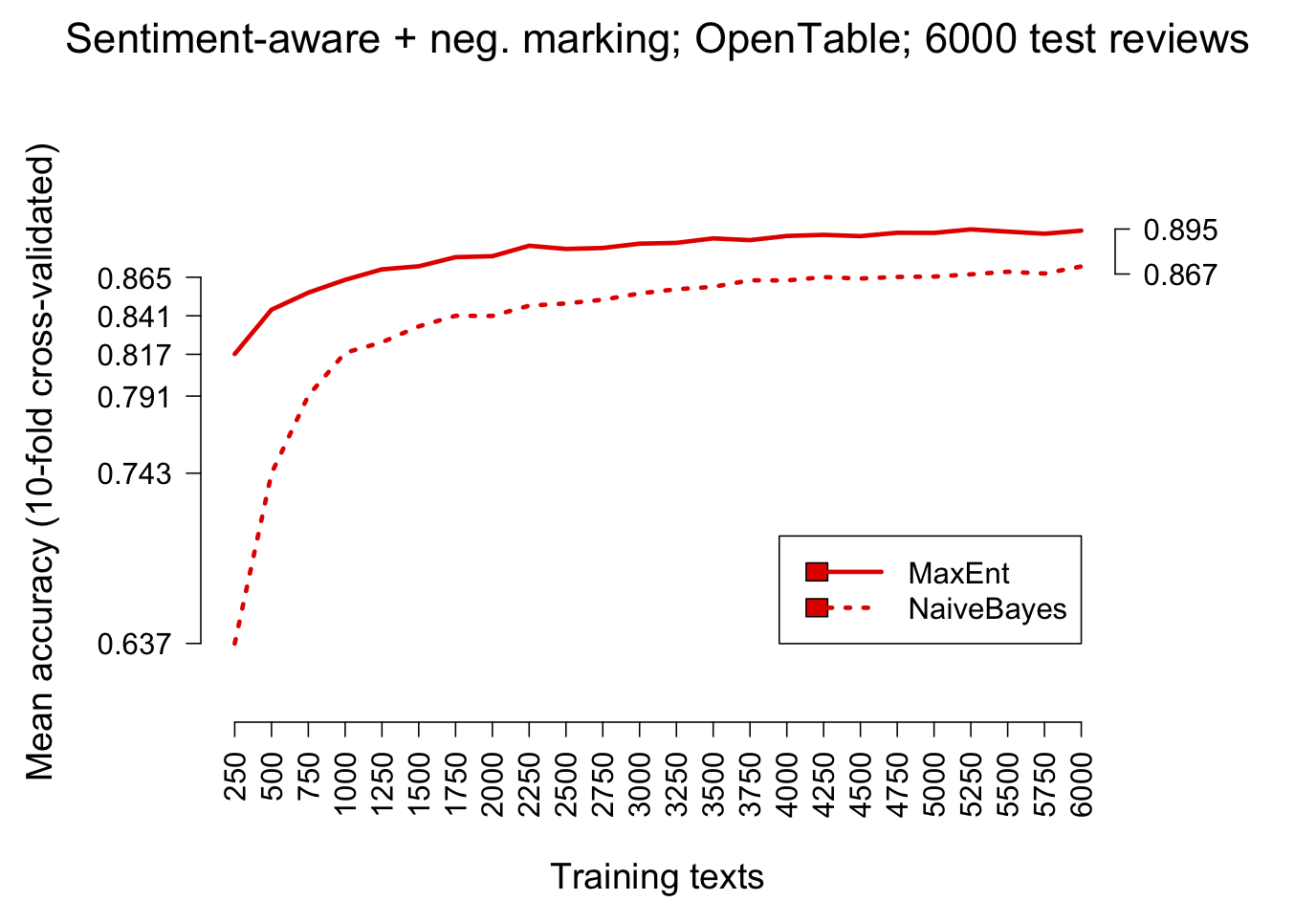
I work with balanced sets throughout, which means that we can safely use accuracy (which in turn greatly simplifies the assessments in general)

On in-domain testing, the MaxEnt model is substantially better than the Naive Bayes model for all of the tokenization schemes we explored earlier. Figure fig:modelcmp_opentable and Figure fig:modelcmp_ep support this claim. The first uses OpenTable data, and the second uses a subset of the Experience Project data for which there is a majority label, which is then treated as the true label for the text.

Figure fig:modelcmp_opentable

MaxEnt and Naive Bayes using the tokenization algorithms discussed earlier.

Figure fig:modelcmp_ep

MaxEnt and Naive Bayes using the tokenization algorithms discussed earlier, training and testing Experience Project confessions.

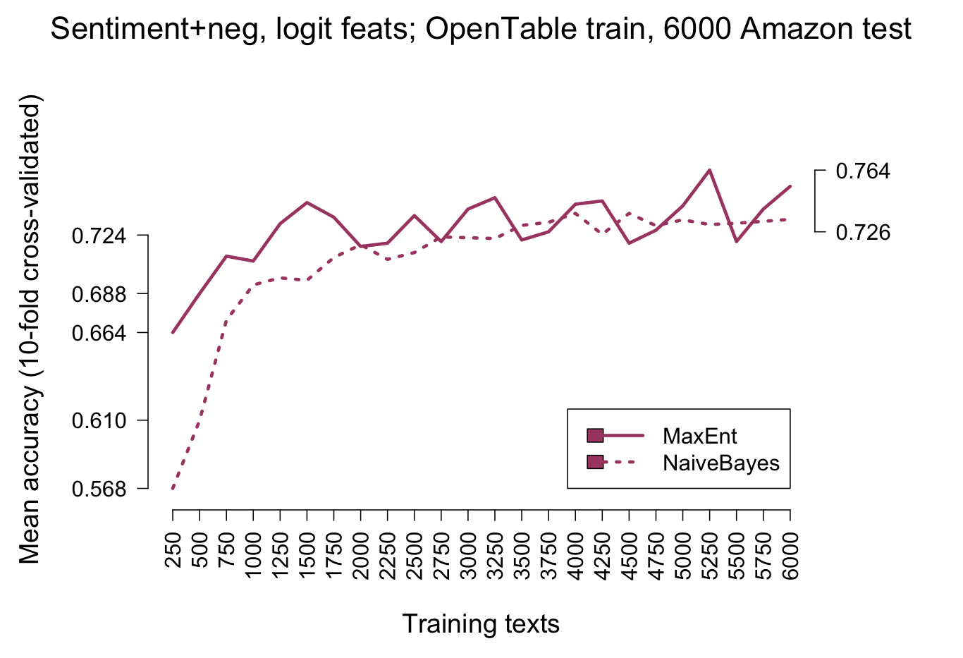
However, he picture is less clear when we move to experiments involving out-of-domain testing. Figure fig:modelcmp_xtrain_imdb and figure fig:modelcmp_xtrain_amazon report on such comparisons. In both cases, we train on OpenTable data. Figure fig:modelcmp_xtrain_imdb tests the model on IMDB data, and figure fig:modelcmp_xtrain_amazon tests it on Amazon reviews. In both cases, though MaxEnt does really well with small amounts of data, it is quickly outdone by the Naive Bayes model.

Figure fig:modelcmp_xtrain_imdb

MaxEnt and Naive Bayes using the tokenization algorithms discussed earlier, training and testing on different domains.

Figure fig:modelcmp_xtrain_amazon

MaxEnt and Naive Bayes using the tokenization algorithms discussed earlier, training and testing on different domains.

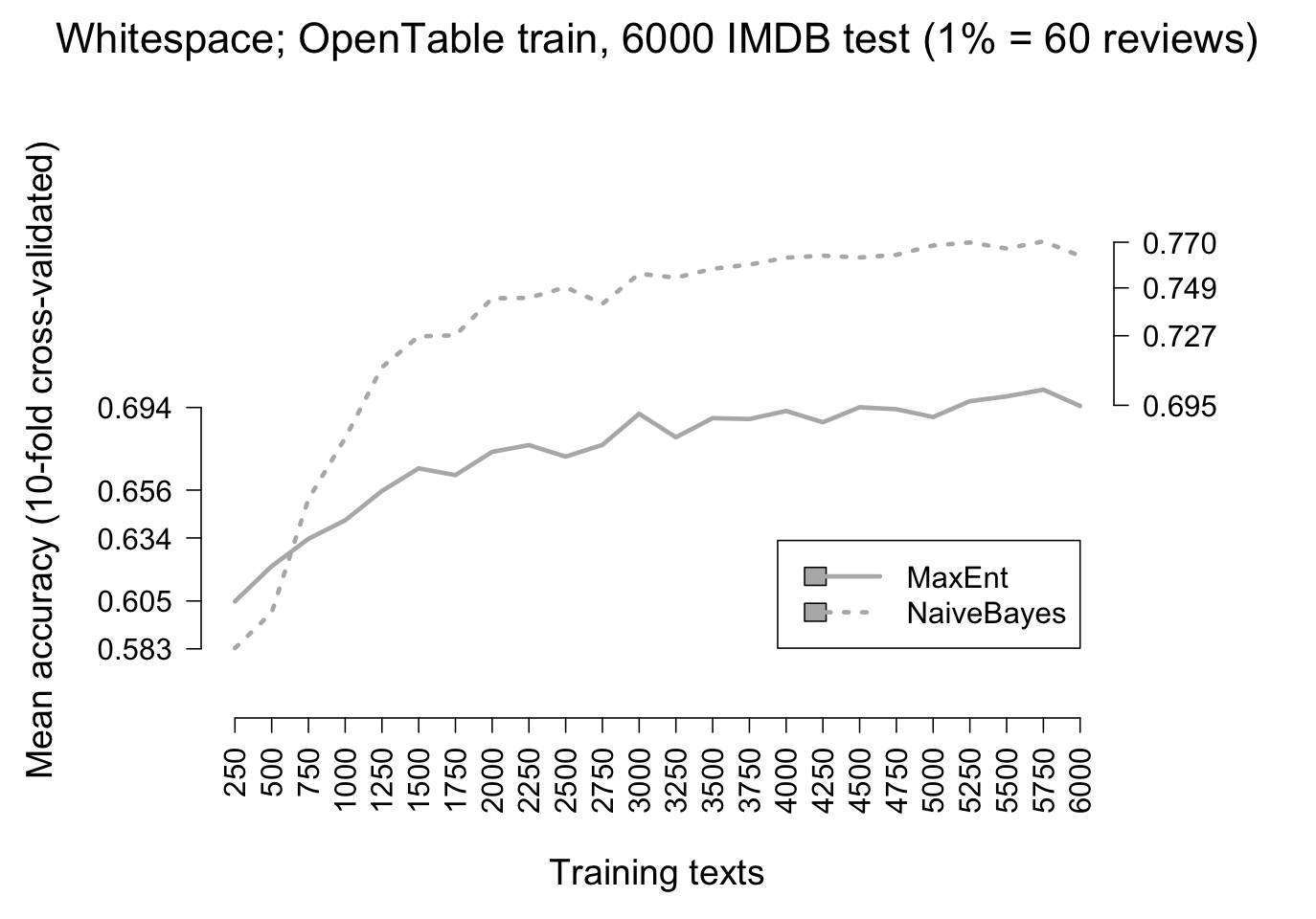
Why is this so? Does it indicate that the Naive Bayes model is actually superior? After all, we typically do not want to make predictions about data that we already have labels for, but rather we want to project those labels onto new data, so we should favor the best out-of-domain model.

Before we make this conclusion, I think we need to do a bit more investigation.

The first step is to see how the models perform on their own training data. Figure fig:traineval presents these experiments. Strinkingly, the MaxEnt model invariably gets 100% of the training data right. Since we are nowhere near that number even on in-domain test sets, it is likely that we are massively overfitting to the training data. This suggests that we should look to sparser feature sets, so that the model generalizes better.

Figure fig:traineval

MaxEnt and Naive Bayes using the tokenization algorithms discussed earlier, testing on the training data.

Feature selection

A priori method cut-offs

Probably the most common method for reducing the size of the feature space is to pick the top N(%) of the features as sorted by overall frequency. The top J features might be removed as well, on the assumption that they are all stopwords that say little about a document's class.

The major drawback to this method is that is can can lose a lot of important sentiment information. Below the N cut-off, there might be infrequent but valuable words like lackluster and hesitant. In the top J are likely to be negation, demonstratives, and personal pronouns that carry subtle but extremely reliable sentiment information (Constant et al. 2008, Potts, Chung and Pennebaker 2007).

Lexicon induction as feature set induction

Where there is metadata, methods like those we employed in the lexicon section for review data and socia networking data can be employed. This basically means restricting attention to the features that have an interesting relationship to the metadata in question. This can be extremely effective in practice. The drawback I see is that you might be limiting the classifier's ability to generalize to out-of-domain data, where the associations might be different. It is possible to address this using the unsupervised methods discussed in the vector-space section, which can enable you to expand your initial lexicon to include more general associations.

Mutual information

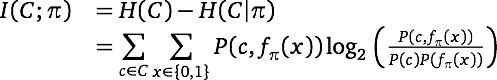
Another way to leverage one's labels to good effect is to pick the top N features as ranked not by frequency but rather by mutual information with the class labels (McCallum and Nigam 1998):

Definition: Mutual information between features and class labels

A cautionary note

Pang and Lee present evidence that sentiment classifier accuracy increases steadily with the size of the vocabulary. We actually already saw a glimpse of this in the Language and Cognition section; the relevant figure is repeated as figure fig:others. However, the ever-better models we get are likely to have trouble generalizing to new data. Thus, despite the risks, some kind of reduction in the feature space is likely to pay off.

Figure fig:others

A single classifier model (MaxEnt) applied to three different domains at various vocabulary sizes, with vocabulary selection done by mutual information with the class labels.

Back the model competition

To recap, we've discovered that the MaxEnt model is over-fitting to the training data, which is hurting its out-of-domain performance. The hypothesis is that if we reduce the feature space, the MaxEnt model will pull ahead of the Naive Bayes model even for out-of-domain testing. (Recall that it is already significantly better for in-domain testing.)

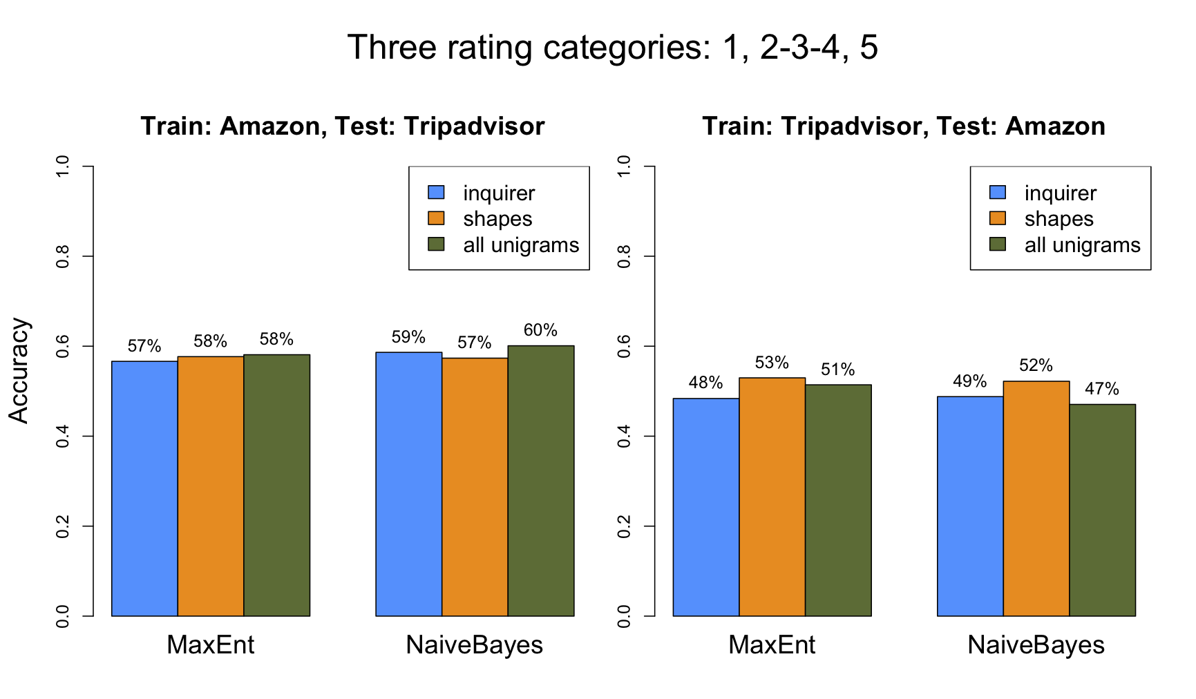
Figure fig:selected reports on experiments along these lines. Both models are largely improved by reduced features space, but MaxEnt really pulls ahead pretty decisively when one looks at the overall performance numbers.

Figure fig:selected

Model comparison for a feature set derived via the lexicon induction method of the IMDB lexicon section. The smaller model addresses the over-fitting problem for MaxEnt, allowing it to pull ahead of Naive Bayes. I am not sure why the MaxEnt performance is so volatile, though. I've included results from earlier, different experiments to try to make the overall picture clearer.

Tools

There are excellent software packages available for fitting models like these. This section focusses on the Stanford Classifier but links to others that are also extremely useful.

The Stanford Classifier

The Stanford Classifier is written in Java, and the distribution provides example code for integrating it into your own projects. It is free for academic use, and the licensing fees for commerical use are very reasonable.

The classifier also has an excellent command-line interface. One simply creates tab-separated training and testing files. One column (usually the leftmost, or 0th) provides the true labels. The remaining columns specify features, which can be boolean, integer, real-valued, or textual. For textual columns, one can specify how to break it up into string-based boolean features.

The command-line interface is fully documented in the javadoc/ directory of the classifier distribution: open index.html in a Web browser and find ColumnDataClassifier in the lower-left navigation bar.

Figure fig:propfile contains a prop (properties) file for the classifier.

# USAGE
# java -mx3000m -jar stanford-classifier.jar -prop $THISFILENAME
#
##### Training and testing source, as tab-separated-values files:
#
trainFile=$TRAINFILE.tsv
testFile=$TESTFILE.tsv
#
# Model (useNB=false is MaxEnt; useNB=true is NaiveBayes)
useNB=false
#
##### Features
#
# Use the class feature to capture any biases coming 
# from imbalanced class sizes:
#
useClassFeature=true
#
# The true class labels are given in column 0 (leftmost)
#
goldAnswerColumn=0
#
# Suppose that column 1 contains something like the frequency 
# of sentiment words overall. We tell the classifier to treat 
# the values as numeric and to log-transform them:
1.realValued=true
1.logTransform=true
#
# Column 2 contains our textual features, already tokenized. 
# This says that column 1 is text in which the tokens are 
# separated by |||. use splitWordsRegexp=\\s+ to split on 
# whitespace
#
2.useSplitWords=true
2.splitWordsRegexp=\\|\\|\\|
#
# Don't display a column to avoid screen clutter; 
# use positive numbers to pick out columns you want displayed:
#
displayedColumn=-1
#
# Output a complete representation of the model to a file:
#
printClassifier=AllWeights
printTo=$CLASSIFIERFILE
#
# These are the recommended optimization parameters for MaxEnt; 
# if useNB=true, they are ignored:
#
prior=quadratic
intern=true
sigma=1.0
useQN=true
QNsize=15
tolerance=1e-4

Others

• MALLET (Java): flexible command-line interface; fully extendible; implements a wide range of classifier; excellent facilities for cross-validation and out-of-domain testing; also provides many other NLP tools, including topic models and optimization methods.
• NLTK (Python): very flexible Naive Bayes and MaxEnt implementations.
• LingPipe (Java): lots of different classifier models, some of them highly tuned for specific linguistic applications (including sentiment)

A lightweight, accurate classifier

The models discussed above tend to be costly in terms of the disk space, memory, and time they require for both training and prediction.

Here's a proposal for how to build a lightweight, accurate classifier that is quick to train on even hundreds of thousands of instances, and that makes predictions for new texts in well under a second:

1. Begin with a set of N fixed sentiment lexicons L. For my experiments, I used the fixed polarity lexicons, the IMDB scores, the Experience Project O/E vectors, and the sentiment-rich classes from the Harvard General Inquirer and LIWC. The total number of predictors was 39, all of them numeric.
2. The feature function tokenizes each text using the sentiment-aware tokenizer with negation marking. _NEG marked phrases have scores in the IMDB and EP data, and are treated like their unmarked counterparts by the other lexicons.
3. For a given text, the feature function simply sums up all the words' scores for each of the 39 predictors and then normalizes them by the length of the text. Thus, each text is modeled as a vector of 39 numbers.
4. Trained and evaluate MaxEnt models to assess performance.

A summary of the experiments I did is given in table tab:lightweight. Overall, the performance is highly competitive with state-of-the-art classifiers, and the model does almost no-overfitting. (Indeed, we could probably stand to fit more tightly to the training data.)

Summary of conclusions

1. Accuracy numbers are meaningful only to the extent that the test set is balanced. Where it is imbalanced, precision and recall number are better.
2. Watch out for over-fitting. A model that does beautifully in-domain might fall apart out of domain. The problem is especially pressing for MaxEnt, which has the power to memorize large training sets.
3. Favor feature selection functions that are sensitive to what is happening in the training data.
4. On the whole, MaxEnt is an improvement over Naive Bayes: MaxEnt is more flexible in terms of its features, and it deals better with correlated features.